Tag Archives | process

NumPy where tutorial (With Examples)

Looking up for entries that satisfy a specific condition is a painful process, especially if you are searching it in a large dataset having hundreds or thousands of entries. If you know the fundamental SQL queries, you must be aware of the ‘WHERE’ clause that is used with the SELECT statement to fetch such entries from a relational database that satisfy certain conditions. NumPy offers similar functionality to find such items in a NumPy array that satisfy a given Boolean condition through its ‘where()‘ function — except that it is used in a slightly different way than the SQL SELECT statement with the WHERE clause. In this tutorial, we’ll look at the various ways the NumPy where function can be used for a variety of use cases. Let’s get going.

Continue Reading →

A very simple usage of NumPy where

Let’s begin with a simple application of ‘np.where()‘ on a 1-dimensional NumPy array of integers.
We will use ‘np.where’ function to find positions with values that are less than 5.

We’ll first create a 1-dimensional array of 10 integer values randomly chosen between 0 and 9.

import numpy as np

np.random.seed(42)

a = np.random.randint()

print("a = {}".format(a))

Output:

a = [6 3 7 4 6 9 2 6 7 4]

Now we will call ‘np.where’ with the condition ‘a < 5’ i.e we’re asking ‘np.where’ to tell us where in the array a are the values less than 5. It will return us an array of indices where the specified condition is satisfied.

result = np.where(a < 5)

print(result)

Output:

(array([1, 3, 6, 9]),)

We get the indices 1,3,6,9 as output and it can be verified from the array that the values at these positions are indeed less than 5.
Note that the returned value is a 1-element tuple. This tuple has an array of indices.
We’ll understand the reason for the result being returned as a tuple when we discuss np.where on 2D arrays.

How does NumPy where work?

To understand what goes on inside the complex expression involving the ‘np.where’ function, it is important to understand the first parameter of ‘np.where’, that is, the condition.

When we call a Boolean expression involving NumPy array such as ‘a > 2’ or ‘a % 2 == 0’, it actually returns a NumPy array of Boolean values.

This array has the value True at positions where the condition evaluates to True and has the value False elsewhere. This serves as a ‘mask‘ for NumPy where function.

Here is a code example.

a = np.array([1, 10, 13, 8, 7, 9, 6, 3, 0])

print ("a > 5:")

print(a > 5)

Output:

a > 5:
[false True True True True True True False False]

So what we effectively do is that we pass an array of Boolean values to the ‘np.where’ function which then returns the indices where the array had the value True.

This can be verified by passing a constant array of Boolean values instead of specifying the condition on the array that we usually do.

bool_array = np.array([True, True, True, False, False, False, False, False, False])

print(np.where(bool_array)

Output:

(array([0, 1, 2]),)

Notice how, instead of passing a condition on an array of actual values, we passed a Boolean array and the ‘np.where’ function returned us the indices where the values were True.

2D matrices

Now that we have seen it on 1-dimensional NumPy arrays, let us understand how would ‘np.where’ behave on 2D matrices.

The idea remains the same. We call the ‘np.where’ function and pass a condition on a 2D matrix. The difference is in the way it returns the result indices.
Earlier, np.where returned a 1-dimensional array of indices (stored inside a tuple) for a 1-D array, specifying the positions where the values satisfy a given condition.

But in the case of a 2D matrix, a single position is specified using 2 values — the row index and the column index.
So in this case, np.where will return 2 arrays, the first one carrying the row indices and the second one carrying the corresponding column indices.

Both these rows and column index arrays are stored inside a tuple (now you know why we got a tuple as an answer even in case of a 1-D array).

Let’s see this in action to better understand it.
We’ll write a code to find where in a 3×3 matrix are the entries divisible by 2.

np.random.seed(42)

a = np.random.randint(0,10, size=(3,3))

print("a =\n{}\n".format(a))

result = np.where(a % 2 == 0)

print("result: {}".format(result))

Output:

a =
[[6 3 7]
[4 6 9]
[2 6 7]

result: (array([0, 1, 1, 2, 2]], array([0, 0, 1, 0, 1]))

The returned tuple has 2 arrays, each bearing the row and column indices of the positions in the matrix where the values are divisible by 2.

Ordered pairwise selection of values from the two arrays gives us a position each.
The length of each of the two arrays is 5, indicating there are 5 such positions satisfying the given condition.

If we look at the 3rd pair — (1,1), the value at (1,1) in the matrix is 6 which is divisible by 2.
Likewise, you can check and verify with other pairs of indices as well.

Multidimensional array

Just as we saw the working of ‘np.where’ on a 2-D matrix, we will get similar results when we apply np.where on a multidimensional NumPy array.

The length of the returned tuple will be equal to the number of dimensions of the input array.
Each array at position k in the returned tuple will represent the indices in the kth dimension of the elements satisfying the specified condition.

Let’s quickly look at an example.

np.random.seed(42)

a = np.random.randint(0,10, size=(3,3,3,3)) #4-dimensional array

print("a =\n{}\n".format(a))

result = np.where(a == 5) #checking which values are equal to 5

print("len(result)= {}".format(len(result)))

print("len(result[0]= {})".format(len(result[0])))

Output:

len(result) = 4 indicates the input array is of 4 dimension.

The length of one of the arrays in the result tuple is 6, which means there are six positions in the given 3x3x3x3 array where the given condition (i.e containing value 5) is satisfied.

Using the result as an index

So far we have looked at how we get the tuple of indices, in each dimension, of the values satisfying the given condition.

Most of the time we’d be interested in fetching the actual values satisfying the given condition instead of their indices.

To achieve this, we can use the returned tuple as an index on the given array. This will return only those values whose indices are stored in the tuple.

Let’s check this for the 2-D matrix example.

np.random.seed(42)

a = np.random.randint(0,10, size=(3,3))

print("a =\n{}\n".format(a))

result_indices = np.where(a % 2 == 0)

result = a[result_indices]

print("result: {}".format(result))

Output:

a =
[[6 3 7]
[4 6 9]
[2 6 7]]

result: [6 4 6 2 6]

As discussed above, we get all those values (not their indices) that satisfy the given condition which, in our case, was divisibility by 2 i.e even numbers.

Parameters ‘x’ and ‘y’

Instead of getting the indices as a result of calling the ‘np.where’ function, we can also provide as parameters, two optional arrays x and y of the same shape (or broadcastable shape) as input array, whose values will be returned when the specified condition on the corresponding values in input array is True or False respectively.

For instance, if we call the method on a 1-dimensional array of length 10, and we supply two more arrays x and y of the same length.
In this case, whenever a value in input array satisfies the given condition, the corresponding value in array x will be returned whereas, if the condition is false on a given value, the corresponding value from array y will be returned.

These values from x and y at their respective positions will be returned as an array of the same shape as the input array.

Let’s get a better understanding of this through code.

np.random.seed(42)

a = np.random.randint(0,10, size=(10))

x = a

y = a*10

print("a = {}".format(a))

print("x = {}".format(x))

print("y = {}".format(y))

result = np.where(a%2 == 1, x, y) #if number is odd return the same number else return its multiple of 10.

print("\nresult = {}".format(result))

Output:

This method is useful if you want to replace the values satisfying a particular condition by another set of values and leaving those not satisfying the condition unchanged.
In that case, we will pass the replacement value(s) to the parameter x and the original array to the parameter y.

Note that we can pass either both x and y together or none of them. We can’t pass one of them and skip the other.

Apply on Pandas DataFrames

Numpy’s ‘where’ function doesn’t necessarily have to be applied to NumPy arrays. It can be used with any iterable that would yield a list of Boolean values.

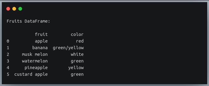
Let us see how we can apply the ‘np.where’ function on a Pandas DataFrame to see if the strings in a column contain a particular substring.

import pandas as pd

import numpy as np

df = pd.DataFrame({"fruit":["apple", "banana", "musk melon",
"watermelon", "pineapple", "custard apple"],
"color": ["red", "green/yellow", "white",
"green", "yellow", "green"]})

print("Fruits DataFrame:\n")

print(df)

Output:

Now we’re going to use ‘np.where’ to extract those rows from the DataFrame ‘df’ where the ‘fruit’ column has the substring ‘apple’

apple_df = df.iloc[np.where(df.fruit.str.contains("apple"))]

print(apple_df)

Output:

Let’s try one more example on the same DataFrame where we extract rows for which the ‘color’ column does not contain the substring ‘yell’.

Note: we use the tilde (~) sign to inverse Boolean values in Pandas DataFrame or a NumPy array.


non_yellow_fruits = df.iloc[np.where(~df.color.str.contains("yell"))]

print("Non Yellow fruits:\n{}".format(non_yellow_fruits))

Output:

Multiple conditions

So far we have been evaluating a single Boolean condition in the ‘np.where’ function. We may sometimes need to combine multiple Boolean conditions using Boolean operators like ‘AND‘ or ‘OR’.

It is easy to specify multiple conditions and combine them using a Boolean operator.
The only caveat is that for the NumPy array of Boolean values, we cannot use the normal keywords ‘and’ or ‘or’ that we typically use for single values.
We need to use the ‘&’ operator for ‘AND’ and ‘|’ operator for ‘OR’ operation for element-wise Boolean combination operations.

Let us understand this through an example.

np.random.seed(42)

a = np.random.randint(0,15, (5,5)) #5x5 matrix with values from 0 to 14

print(a)

Output:

We will look for values that are smaller than 8 and are odd. We can combine these two conditions using the AND (&) operator.

# get indices of odd values less than 8 in a
indices = np.where((a < 8) & (a % 2==1))

#print the actual values
print(a[indices])

Output:

We can also use the OR (|) operator to combine the same conditions. This will give us values that are ‘less than 8’ OR ‘odd values’ i.e all values less than 8 and all odd values greater than 8 will be returned.

# get indices of values less than 8 OR odd values in a
indices = np.where((a < 8) | (a % 2==1))

#print the actual values
print(a[indices])

Output:

Nested where (where within where)

Let us revisit the example of our ‘fruits’ table.


import pandas as pd

import numpy as np

df = pd.DataFrame({"fruit":["apple", "banana", "musk melon",
"watermelon", "pineapple", "custard apple"],
"color": ["red", "green/yellow", "white",
"green", "yellow", "green"]})

print("Fruits DataFrame:\n")

print(df)

Output:

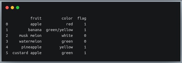
Now let us suppose we wanted to create one more column ‘flag’ which would have the value 1 if the fruit in that row has a substring ‘apple’ or is of color ‘yellow’. We can achieve this by using nested where calls i.e we will call ‘np.where’ function as a parameter within another ‘np.where’ call.

df['flag'] = np.where(df.fruit.str.contains("apple"), 1, # if fruit == 'apple', set 1
np.where(df.color.str.contains("yellow"), 1, 0)) #else if color has 'yellow' set 1, else set 0

print(df)

Output:

The complex expression above can be translated into simple English as:

  1. If the ‘fruit’ column has the substring ‘apple’, set the ‘flag’ value to 1
  2. Else:
    1. If the ‘color’ column has substring ‘yellow’, set the ‘flag’ value to 1
    2. Else set the ‘flag’ value to 0

Note that we can achieve the same result using the OR (|) operator.

#set flag = 1 if any of the two conditions is true, else set it to 0
df['flag'] = np.where(df.fruit.str.contains("apple") |
df.color.str.contains("yellow"), 1, 0)

print(df)

Output:

Thus nested where is particularly useful for tabular data like Pandas DataFrames and is a good equivalent of the nested WHERE clause used in SQL queries.

Finding rows of zeros

Sometimes, in a 2D matrix, some or all of the rows have all values equal to zero. For instance, check out the following NumPy array.

a = np.array([[1, 2, 0],
[0, 9, 20],
[0, 0, 0],
[3, 3, 12],
[0, 0, 0]
[1, 0, 0]])
print(a)

Output:

As we can see the rows 2 and 4 have all values equal to zero. But how do we find this using the ‘np.where’ function?

If we want to find such rows using NumPy where function, we will need to come up with a Boolean array indicating which rows have all values equal to zero.

We can use the ‘np.any()‘ function with ‘axis = 1’, which returns True if at least one of the values in a row is non-zero.

The result of np.any() will be a Boolean array of length equal to the number of rows in our NumPy matrix, in which the positions with the value True indicate the corresponding row has at least one non-zero value.

But we needed a Boolean array that was quite the opposite of this!

That is, we needed a Boolean array where the value ‘True’ would indicate that every element in that row is equal to zero.

Well, this can be obtained through a simple inversion step. The NOT or tilde (~) operator inverts each of the Boolean values in a NumPy array.

The inverted Boolean array can then be passed to the ‘np.where’ function.

Ok, that was a long, tiring explanation.
Let’s see this thing in action.

zero_rows = np.where(~np.any(a, axis=1))[0]

print(zero_rows)

Output:

Let’s look at what’s happening step-by-step:

  1. np.any() returns True if at least one element in the matrix is True (non-zero). axis = 1 indicates it to do this operation row-wise.
  2. It would return a Boolean array of length equal to the number of rows in a, with the value True for rows having non-zero values, and False for rows having all values = 0.
    np.any(a, axis=1)
    Output:

3.The tilde (~) operator inverts the above Boolean array:
~np.any(a, axis=1)
Output:

  1. ‘np.where()’ accepts this Boolean array and returns indices having the value True.

The indexing [0] is used because, as discussed earlier, ‘np.where’ returns a tuple.

Finding the last occurrence of a true condition

We know that NumPy’s ‘where’ function returns multiple indices or pairs of indices (in case of a 2D matrix) for which the specified condition is true.

But sometimes we are interested in only the first occurrence or the last occurrence of the value for which the specified condition is met.

Let’s take the simple example of a one-dimensional array where we will find the last occurrence of a value divisible by 3.

np.random.seed(42)

a = np.random.randint(0,10, size=(10))

print("Array a:", a)

indices = np.where(a%3==0)[0]

last_occurrence_position = indices[-1]

print("last occurrence at", last_occurrence_position)

Output:

Here we could directly use the index ‘-1’ on the returned indices to get the last value in the array.

But how would we extract the position of the last occurrence in a multidimensional array, where the returned result is a tuple of arrays and each array stores the indices in one of the dimensions?

We can use the zip function which takes multiple iterables and returns a pairwise combination of values from each iterable in the given order.

It returns an iterator object, and so we need to convert the returned object into a list or a tuple or any iterable.

Let’s first see how zip works:


a = (1, 2, 3, 4)

b = (5, 6, 7, 8)

c = list(zip(a,b))

print(c)

Output:

So the first element of a and the first element of b form a tuple, then the second element of a and the second element of b form the second tuple in c, and so on.

We’ll use the same technique to find the position of the last occurrence of a condition being satisfied in a multidimensional array.

Let’s use it for a 2D matrix with the same condition as we saw in the earlier example.

np.random.seed(42)

a = np.random.randint(0,10, size=(3,3))

print("Matrix a:\n", a)

indices = np.where(a % 3 == 0)

last_occurrence_position = list(zip(*indices))[-1]

print("last occurrence at",last_occurrence_position)

Output:

We can see in the matrix the last occurrence of a multiple of 3 is at the position (2,1), which is the value 6.

Note: The * operator is an unpacking operator that is used to unpack a sequence of values into separate positional arguments.

Using on DateTime data

We have been using ‘np.where’ function to evaluate certain conditions on either numeric values (greater than, less than, equal to, etc.), or string data (contains, does not contain, etc.)

We can also use the ‘np.where’ function on datetime data.

For example, we can check in a list of datetime values, which of the datetime instances are before/after a given specified datetime.

Let’s understand this through an example.
Note: We’ll use Python’s datetime module to create date objects.

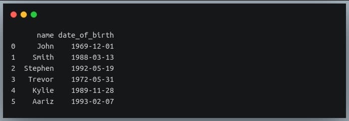
Let’s first define a DataFrame specifying the dates of birth of 6 individuals.

import datetime

names = ["John", "Smith", "Stephen", "Trevor", "Kylie", "Aariz"]

dob = [datetime.datetime(1969, 12, 1),
datetime.datetime(1988, 3, 13),
datetime.datetime(1992, 5, 19),
datetime.datetime(1972, 5, 31),
datetime.datetime(1989, 11, 28),
datetime.datetime(1993, 2, 7)]

data_birth = pd.DataFrame({"name":names, "date_of_birth":dob})

print(data_birth)

Output:

This table has people from diverse age groups!
Let us now specify a condition where we are interested in those individuals who are born on or post-January 1, 1990.

post_90_indices = np.where(data_birth.date_of_birth >= '1990-01-01')[0]

print(post_90_indices)

Output:

Rows 2 and 5 have Smith and Kylie who are born in the years 1992 and 1993 respectively.

Here we are using the ‘greater than or equal to’ (>=) operator on a datetime data, which we generally use with numeric data.
This is possible through operator overloading.

Let’s try one more example. Let’s fetch individuals that were born in May.
Note: Pandas Series provides ‘dt’ sub-module for datetime specific operations, similar to the ‘str’ sub-module we saw in our earlier examples.

may_babies = data_birth.iloc[np.where(data_birth.date_of_birth.dt.month == 5)]

print("May babies:\n{}".format(may_babies))

Output:

Conclusion

We began the tutorial with simple usage of ‘np.where’ function on a 1-dimensional array with conditions specified on numeric data.

We then looked at the application of ‘np.where’ on a 2D matrix and then on a general multidimensional NumPy array.
We also understood how to interpret the tuple of arrays returned by ‘np.where’ in such cases.

We then understood the functionality of ‘np.where’ in detail, using Boolean masks.
We also saw how we can use the result of this method as an index to extract the actual original values that satisfy the given condition.

We looked at the behavior of the ‘np.where’ function with the optional arguments ‘x’ and ‘y’.

We then checked the application of ‘np.where’ on a Pandas DataFrame, followed by using it to evaluate multiple conditions.

We also looked at the nested use of ‘np.where’, its usage in finding the zero rows in a 2D matrix, and then finding the last occurrence of the value satisfying the condition specified by ‘np.where’

Finally, we used ‘np.where’ function on a datetime data, by specifying chronological conditions on a datetime column in a Pandas DataFrame.

0

20+ examples for NumPy matrix multiplication

In this tutorial, we will look at various ways of performing matrix multiplication using NumPy arrays. we will learn how to multiply matrices with different sizes together. Also. we will learn how to speed up the multiplication process using GPU and other hot topics, so let’s get started! Before we move ahead, it is better to review some basic terminologies of Matrix Algebra. Basic Terminologies: Vector: Algebraically, a vector is a collection of coordinates of a point in space. Thus, a vector with 2 values represents a point in a 2-dimensional space. In Computer Science, a vector is an arrangement of numbers along a single dimension. It is also commonly known as an array or a list or a tuple. Eg. [1,2,3,4] Matrix: A matrix (plural matrices) is a 2-dimensional arrangement of numbers or a collection of vectors.

Continue Reading →

Ex:

[[1,2,3],
[4,5,6],
[7,8,9]]

Dot Product: A dot product is a mathematical operation between 2 equal-length vectors.
It is equal to the sum of the products of the corresponding elements of the vectors.
vector dot product operation

With a clear understanding of these terminologies, we are good to go.

Matrix multiplication with a vector

Let’s begin with a simple form of matrix multiplication – between a matrix and a vector.

Before we proceed, let’s first understand how a matrix is represented using NumPy.

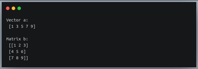
NumPy’s array() method is used to represent vectors, matrices, and higher-dimensional tensors. Let’s define a 5-dimensional vector and a 3×3 matrix using NumPy.

import numpy as np

a = np.array([1, 3, 5, 7, 9])

b = np.array([[1, 2, 3],
[4, 5, 6],
[7, 8, 9]])

print("Vector a:\n", a)

print()

print("Matrix b:\n", b)

Output:

Let us now see how multiplication between a matrix and a vector takes place.

The following points should be kept in mind for a matrix-vector multiplication:

  1. The result of a matrix-vector multiplication is a vector.
  2. Each element of this vector is got by performing a dot product between each row of the matrix and the vector being multiplied.
  3. The number of columns in the matrix should be equal to the number of elements in the vector.

matrix vector multiplication
We’ll use NumPy’s matmul() method for most of our matrix multiplication operations.
Let’s define a 3×3 matrix and multiply it with a vector of length 3.

import numpy as np

a = np.array([[1, 2, 3],
[4, 5, 6],
[7, 8, 9]])
b= np.array([10, 20, 30])

print("A =", a)

print("b =", b)

print("Ab =",np.matmul(a,b))

Output:

Notice how the result is a vector of length equal to the rows of the multiplier matrix.

Multiplication with another matrix

Now,  we understood the multiplication of a matrix with a vector, it would be easy to figure out the multiplication of two matrices.
But, before that, let’s review the most important rules of matrix multiplication:

  1. The number of columns in the first matrix should be equal to the number of rows in the second matrix.
  2. If we are multiplying a matrix of dimensions m x n with another matrix of dimensions n x p, then the resultant product will be a matrix of dimensions m x p.

Let us consider multiplication of an m x n matrix A with an n x p matrix B: input matrices A and BC, product of A and B
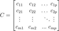
The product of the two matrices C = AB will have m row and p columns.
Each element in the product matrix C results from a dot product between a row vector in A and a column vector in B.

formula for each element in matrix multiplication result
Let us now do a matrix multiplication of 2 matrices in Python, using NumPy.
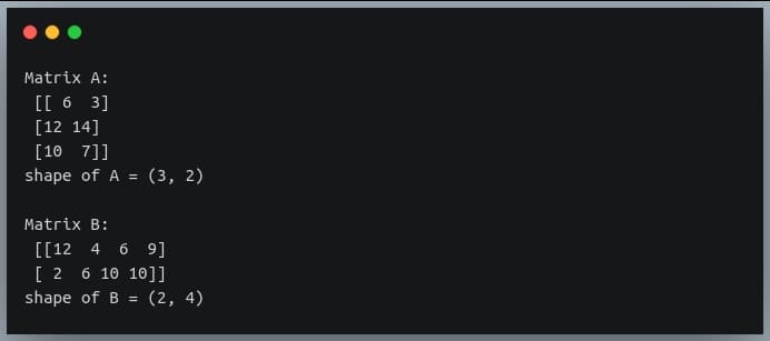
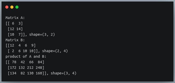
We’ll randomly generate 2 matrices of dimensions 3 x 2 and 2 x 4.
We will use np.random.randint() method to generate the numbers.

import numpy as np

np.random.seed(42)

A = np.random.randint(0, 15, size=(3,2))

B = np.random.randint(0, 15, size =(2,4))

print("Matrix A:\n", A)

print("shape of A =", A.shape)

print()

print("Matrix B:\n", B)

print("shape of B =", B.shape)

Output:

Note: we are setting a random seed using ‘np.random.seed()’ to make the random number generator deterministic.
This will generate the same random numbers each time you run this code snippet. This step is essential if you want to reproduce your result at a later point.

You can set any other integer as seed, but I suggest to set it to 42 for this tutorial so that your output will match the ones shown in the output screenshots.

Let us now multiply the two matrices using the np.matmul() method. The resulting matrix should have the shape 3 x 4.

C = np.matmul(A, B)

print("product of A and B:\n", C)

print("shape of product =", C.shape)

Output:

Multiplication between 3 matrices

Multiplication of the 3 matrices will be composed of two 2-matrix multiplication operations and each of the two operations will follow the same rules as discussed in the previous section.

Let us say we are multiplying 3 matrices A, B, and C; and the product is D = ABC.
Here, the number of columns in A should be equal to the number of rows in B and the number of rows in C should be equal to the number of columns in B.

The resulting matrix will have rows equal to the number of rows in A, and columns equal to the number of columns in C.

An important property of matrix multiplication operation is that it is Associative.
With multi-matrix multiplication, the order of individual multiplication operations does not matter and hence does not yield different results.

For instance, in our example of multiplication of 3 matrices D = ABC, it doesn’t matter if we perform AB first or BC first.

diffrent orderings for multiplication of 3 matrices
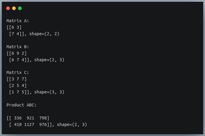
Both orderings would yield the same result. Let us do an example in Python.

import numpy as np

np.random.seed(42)

A = np.random.randint(0, 10, size=(2,2))

B = np.random.randint(0, 10, size=(2,3))

C = np.random.randint(0, 10, size=(3,3))

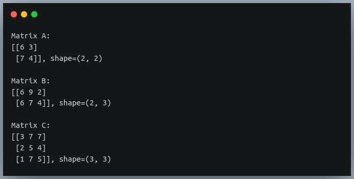
print("Matrix A:\n{}, shape={}\n".format(A, A.shape))

print("Matrix B:\n{}, shape={}\n".format(B, B.shape))

print("Matrix C:\n{}, shape={}\n".format(C, C.shape))

Output:

Based on the rules we discussed above, the multiplication of these 3 matrices should yield a resulting matrix of shape (2, 3).
Note that the method np.matmul() accepts only 2 matrices as input for multiplication, so we will call the method twice in the order that we wish to multiply, and pass the result of the first call as a parameter to the second.
(We’ll find a better way to deal with this problem in a later section when we introduce ‘@’ operator)

Let’s do the multiplication in both orders and validate the property of associativity.

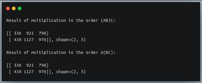
D = np.matmul(np.matmul(A,B), C)

print("Result of multiplication in the order (AB)C:\n\n{},shape={}\n".format(D, D.shape))

D = np.matmul(A, np.matmul(B,C))

print("Result of multiplication in the order A(BC):\n\n{},shape={}".format(D, D.shape))

Output:

As we can see, the result of multiplication of the 3 matrices remains the same whether we multiply A and B first, or B and C first.
Thus, the property of associativity stands validated.
Also, the shape of the resulting array is (2, 3) which is on the expected lines.

NumPy 3D matrix multiplication

A 3D matrix is nothing but a collection (or a stack) of many 2D matrices, just like how a 2D matrix is a collection/stack of many 1D vectors.

So, matrix multiplication of 3D matrices involves multiple multiplications of 2D matrices, which eventually boils down to a dot product between their row/column vectors.

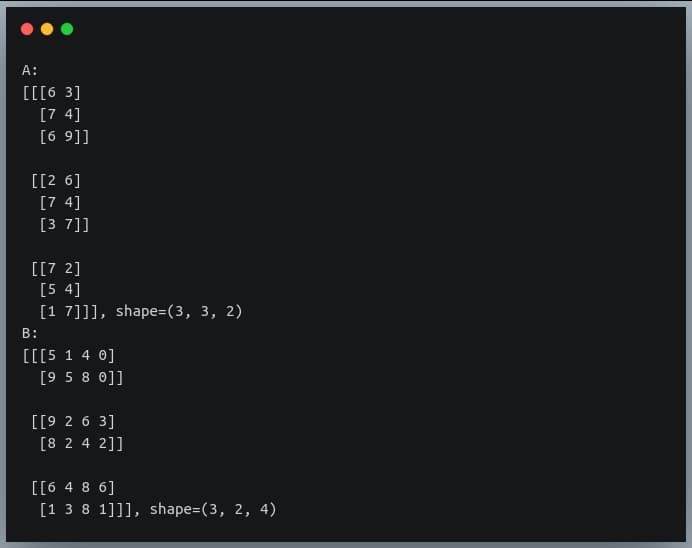
Let us consider an example matrix A of shape (3,3,2) multiplied with another 3D matrix B of shape (3,2,4).

import numpy as np

np.random.seed(42)

A = np.random.randint(0, 10, size=(3,3,2))

B = np.random.randint(0, 10, size=(3,2,4))

print("A:\n{}, shape={}\nB:\n{}, shape={}".format(A, A.shape,B, B.shape))

Output:

The first matrix is a stack of three 2D matrices each of shape (3,2) and the second matrix is a stack of 3 2D matrices, each of shape (2,4).

The matrix multiplication between these two will involve 3 multiplications between corresponding 2D matrices of A and B having shapes (3,2) and (2,4) respectively.

Specifically, the first multiplication will be between A[0] and B[0], the second multiplication will be between A[1] and B[1] and finally, the third multiplication will be between A[2] and B[2].

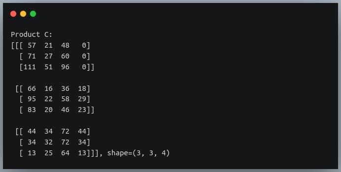
The result of each individual multiplication of 2D matrices will be of shape (3,4). Hence, the final product of the two 3D matrices will be a matrix of shape (3,3,4).

Let’s realize this using code.

C = np.matmul(A,B)

print("Product C:\n{}, shape={}".format(C, C.shape))

Output:

Alternatives to np.matmul()

Apart from ‘np.matmul()’, there are two other ways of doing matrix multiplication – the np.dot() method and the ‘@’ operator, each offering some differences/flexibility in matrix multiplication operations.

The ‘np.dot()’ method

This method is primarily used to find the dot product of vectors, but if we pass two 2-D matrices, then it will behave similarly to the ‘np.matmul()’ method and will return the result of the matrix multiplication of the two matrices.

Let us look at an example:

import numpy as np

# a 3x2 matrix
A = np.array([[8, 2, 2],
[1, 0, 3]])

# a 2x3 matrix
B = np.array([[1, 3],
[5, 0],
[9, 6]])

# dot product should return a 2x2 product
C = np.dot(A, B)

print("product of A and B:\n{} shape={}".format(C, C.shape))

Output:

Here, we defined a 3×2 matrix and a 2×3 matrix and their dot product yields a 2×2 result which is the matrix multiplication of the two matrices,
the same as what ‘np.matmul()’ would have returned.

The difference between np.dot() and np.matmul() is in their operation on 3D matrices.
While ‘np.matmul()’ operates on two 3D matrices by computing matrix multiplication of the corresponding pairs of 2D matrices (as discussed in the last section), np.dot() on the other hand computes dot products of various pairs of row vectors and column vectors from the first and second matrix respectively.

np.dot() on two 3D matrices A and B returns a sum-product over the last axis of A and the second-to-last axis of B.
This is non-intuitive, and not easily comprehensible.

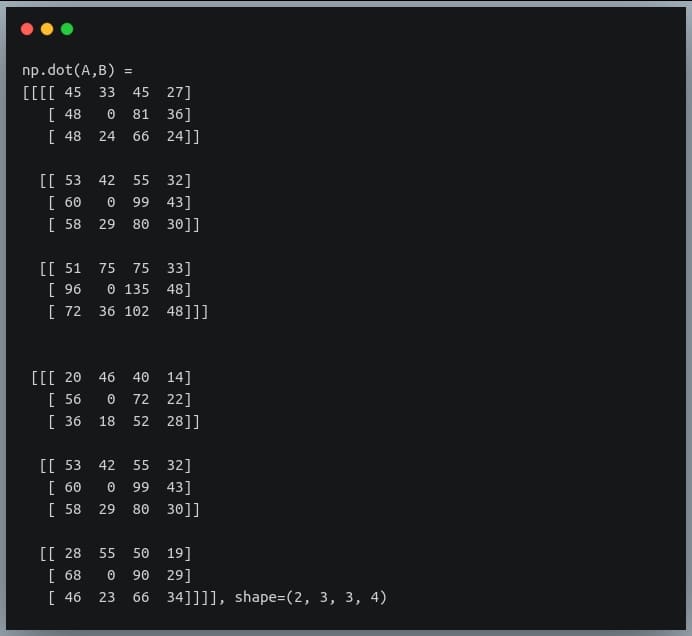
So, if A is of shape (a, b, c) and B is of shape (d, c, e), then the result of np.dot(A, B) will be of shape (a,d,b,e) whose individual element at a position (i,j,k,m) is given by:

dot(A, B)[i,j,k,m] = sum(A[i,j,:] * B[k,:,m])

Let’s check an example:

import numpy as np

np.random.seed(42)

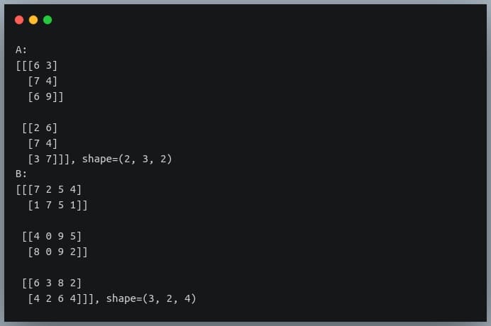
A = np.random.randint(0, 10, size=(2,3,2))

B = np.random.randint(0, 10, size=(3,2,4))

print("A:\n{}, shape={}\nB:\n{}, shape={}".format(A, A.shape,B, B.shape))

Output:

If we now pass these matrices to the ‘np.dot()’ method, it will return a matrix of shape (2,3,3,4) whose individual elements are computed using the formula given above.

C = np.dot(A,B)

print("np.dot(A,B) =\n{}, shape={}".format(C, C.shape))

Output:

Another important difference between ‘np.matmul()’ and ‘np.dot()’ is that ‘np.matmul()’ doesn’t allow multiplication with a scalar (will be discussed in the next section), while ‘np.dot()’ allows it.

The ‘@’ operator

The @ operator introduced in Python 3.5, it performs the same operation as ‘np.matmul()’.

Let’s run through an earlier example of ‘np.matmul()’ using @ operator, and will see the same result as returned earlier:

import numpy as np

np.random.seed(42)

A = np.random.randint(0, 15, size=(3,2))

B = np.random.randint(0, 15, size =(2,4))

print("Matrix A:\n{}, shape={}".format(A, A.shape))

print("Matrix B:\n{}, shape={}".format(B, B.shape))

C = A @ B

print("product of A and B:\n{}, shape={}".format(C, C.shape))

Output:

The ‘@’ operator becomes handy when we are performing matrix multiplication of over 2 matrices.

Earlier, we had to call ‘np.matmul()’ multiple times and pass their results as a parameter to the next call.
Now, we can perform the same operation in a simpler (and a more intuitive) way:

import numpy as np

np.random.seed(42)

A = np.random.randint(0, 10, size=(2,2))

B = np.random.randint(0, 10, size=(2,3))

C = np.random.randint(0, 10, size=(3,3))

print("Matrix A:\n{}, shape={}\n".format(A, A.shape))

print("Matrix B:\n{}, shape={}\n".format(B, B.shape))

print("Matrix C:\n{}, shape={}\n".format(C, C.shape))

D = A @ B @ C # earlier np.matmul(np.matmul(A,B),C)

print("Product ABC:\n\n{}, shape={}\n".format(D, D.shape))

Output:

Multiplication with a scalar (Single value)

So far we’ve performed multiplication of a matrix with a vector or another matrix. But what happens when we perform matrix multiplication with a scalar or a single numeric value?

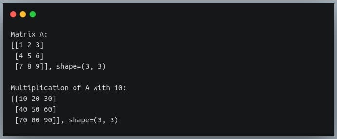
The result of such an operation is got by multiplying each element in the matrix with the scalar value. Thus the output matrix has the same dimension as the input matrix.

Note that ‘np.matmul()’ does not allow the multiplication of a matrix with a scalar. This can be achieved by using the np.dot() method or using the ‘*’ operator.

Let’s see this in a code example.

import numpy as np

A = np.array([[1,2,3],
[4,5, 6],
[7, 8, 9]])

B = A * 10

print("Matrix A:\n{}, shape={}\n".format(A, A.shape))

print("Multiplication of A with 10:\n{}, shape={}".format(B, B.shape))

Output:

Element-wise matrix multiplication

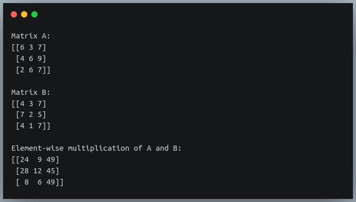
Sometimes we want to do multiplication of corresponding elements of two matrices having the same shape.

element-wise matrix multiplication
This operation is also called as the Hadamard Product. It accepts two matrices of the same dimensions and produces a third matrix of the same dimension.

It can be achieved in Python by calling the NumPy’s multiply() function or using the ‘*’ operator.

import numpy as np

np.random.seed(42)

A = np.random.randint(0, 10, size=(3,3))

B = np.random.randint(0, 10, size=(3,3))

print("Matrix A:\n{}\n".format(A))

print("Matrix B:\n{}\n".format(B))

C = np.multiply(A,B) # or A * B

print("Element-wise multiplication of A and B:\n{}".format(C))

Output:

The only rule to be kept in mind for element-wise multiplication is that the two matrices should have the same shape.
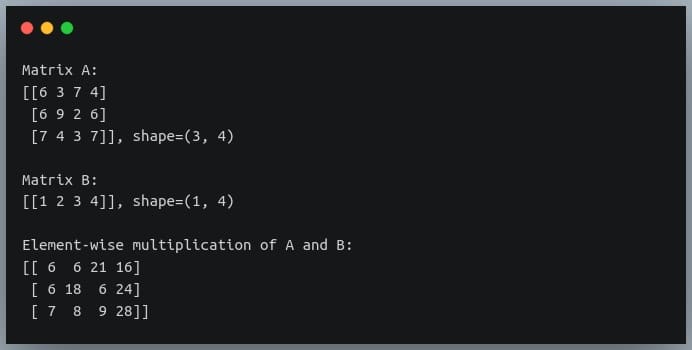
However, if one dimension of a matrix is missing, NumPy would broadcast it to match the shape of the other matrix.

In fact, matrix multiplication with a scalar also involves the broadcasting of the scalar value to a matrix of the shape equal to the matrix operand in the multiplication.

That means when we are multiplying a matrix of shape (3,3) with a scalar value 10, NumPy would create another matrix of shape (3,3) with constant values 10 at all positions in the matrix and perform element-wise multiplication between the two matrices.

Let’s understand this through an example:

import numpy as np

np.random.seed(42)

A = np.random.randint(0, 10, size=(3,4))

B = np.array([[1,2,3,4]])

print("Matrix A:\n{}, shape={}\n".format(A, A.shape))

print("Matrix B:\n{}, shape={}\n".format(B, B.shape))

C = A * B

print("Element-wise multiplication of A and B:\n{}".format(C))

Output:

Notice how the second matrix which had shape (1,4) was transformed into a (3,4) matrix through broadcasting and the element-wise multiplication between the two matrices took place.

Matrix raised to a power (Matrix exponentiation)

Just like how we can raise a scalar value to an exponent, we can do the same operation with matrices.
Just as raising a scalar value (base) to an exponent n is equal to repeatedly multiplying the n bases, the same pattern is observed in raising a matrix to power, which involves repeated matrix multiplications.

For instance, if we raise a matrix A to a power n, it is equal to the matrix multiplications of n matrices, all of which will be the matrix A.

matrix A raised to power n
Note that for this operation to be possible, the base matrix has to be square.
This is to ensure the rules of matrix multiplication are followed (number of columns in preceding matrix = number of rows in the next matrix)

This operation is provided in Python by NumPy’s linalg.matrix_power() method, which accepts the base matrix and an integer power as its parameters.

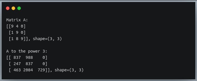
Let us look at an example in Python:

import numpy as np

np.random.seed(10)

A = np.random.randint(0, 10, size=(3,3))

A_to_power_3 = np.linalg.matrix_power(A, 3)

print("Matrix A:\n{}, shape={}\n".format(A, A.shape))

print("A to the power 3:\n{}, shape={}".format(A_to_power_3,A_to_power_3.shape))

Output:

We can validate this result by doing normal matrix multiplication with 3 operands (all of them A), using the ‘@’ operator:

B = A @ A @ A

print("B = A @ A @ A :\n{}, shape={}".format(B, B.shape))

Output:

As you can see, the results from both operations are matching.

An important question that arises from this operation is – What happens when the power is 0?
To answer this question, let us review what happens when we raise a scalar base to power 0.
We get the value 1, right? Now, what is the equivalent of 1 in Matrix Algebra? You guessed it right!

It’s the identity matrix.

So raising an n x n matrix to the power 0 results in an identity matrix I of shape n x n.

Let’s quickly check this in Python, using our previous matrix A.

C = np.linalg.matrix_power(A, 0)

print("A to power 0:\n{}, shape={}".format(C, C.shape))

Output:

Element-wise exponentiation

Just like how we could do element-wise multiplication of matrices, we can also do element-wise exponentiation i.e. raise each individual element of a matrix to some power.

This can be achieved in Python using standard exponent operator ‘**‘ – an example of operator overloading.

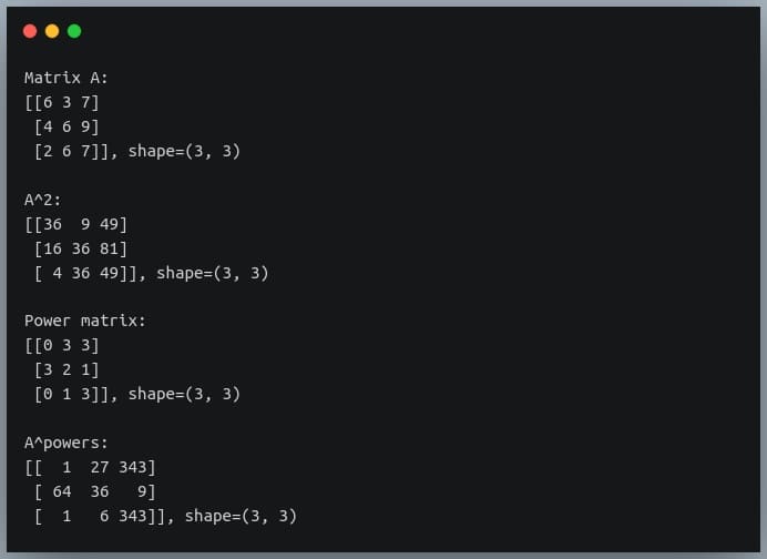
Again, we can provide a single constant power for all the elements in the matrix, or a matrix of powers for each element in the base matrix.

Let’s look at examples of both in Python:

import numpy as np

np.random.seed(42)

A = np.random.randint(0, 10, size=(3,3))

print("Matrix A:\n{}, shape={}\n".format(A, A.shape))

#constant power
B = A**2

print("A^2:\n{}, shape={}\n".format(B, B.shape))

powers = np.random.randint(0, 4, size=(3,3))

print("Power matrix:\n{}, shape={}\n".format(powers, powers.shape))

C = A ** powers

print("A^powers:\n{}, shape={}\n".format(C, C.shape))

Output:

Multiplication from a particular index

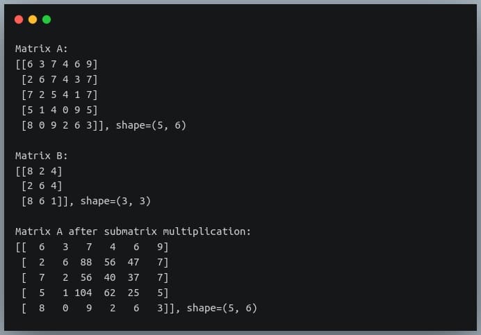
Suppose we have a 5 x 6 matrix A and another 3 x 3 matrix B. Obviously, we cannot multiply these two together, because of dimensional inconsistencies.

But what if we wanted to multiply a 3×3 submatrix in matrix A with matrix B while keeping the other elements in A unchanged?
For better understanding, refer to the following image:

matrix multiplication of A from indices 1,2 to 3,4 with B
This operation can be achieved in Python, by using matrix slicing to extract the submatrix from A, performing multiplication with B, and then writing back the result at relevant index in A.

Let’s see this in action.

import numpy as np

np.random.seed(42)

A = np.random.randint(0, 10, size=(5,6))

B = np.random.randint(0, 10, size=(3,3))

print("Matrix A:\n{}, shape={}\n".format(A, A.shape))

print("Matrix B:\n{}, shape={}\n".format(B, B.shape))

C = A[1:4,2:5] @ B

A[1:4,2:5] = C

print("Matrix A after submatrix multiplication:\n{}, shape={}\n".format(A, A.shape))

Output:

As you can see, only the elements at row indices 1 to 3 and column indices 2 to 4 have been multiplied with B and the same have been written back in A, while the remaining elements of A have remained unchanged.

Also, it’s unnecessary to overwrite the original matrix. We can also write the result in a new matrix, by first copying the original matrix to a new matrix and then writing the product at the position of the submatrix.

Matrix multiplication using GPU
We know that NumPy speeds up the matrix operations by parallelizing a lot of computations and making use of our CPU’s parallel computing capabilities.

However, modern-day applications need more than that. CPUs offer limited computation capabilities, and it does not suffice for the large number of computations that we need, typically in applications like deep learning.

That is where GPUs come into the picture. They offer large computation capabilities and excellent parallelized computation infrastructure, which helps us save a significant amount of time by doing hundreds of thousands of operations within fractions of seconds.

In this section, we will look at how we can perform matrix multiplication on a GPU, instead of a CPU and save a lot of time doing so.

NumPy does not offer the functionality to do matrix multiplications on GPU. So we must install some additional libraries that help us achieve our goal.

We will first install the ‘scikit-cuda‘ and ‘PyCUDA‘ libraries using pip install. These libraries help us perform computations on CUDA based GPUs. To install these libraries from your terminal, if you have a GPU installed on your machine.

pip install pycuda

pip install scikit-cuda

If you do not have a GPU on your machine, you can try out Google Colab notebooks, and enable GPU access, it’s free for use. Now we will write the code to generate two 1000×1000 matrices and perform matrix multiplication between them using two methods:

  1. Using NumPy’s ‘matmul()‘ method on a CPU
  2. Using scikit-cuda’s ‘linalg.mdot()‘ method on a GPU

In the second method, we will generate the matrices on a CPU, then we will store them on GPU (using PyCUDA’s ‘gpuarray.to_gpu()‘ method) before performing the multiplication between them. We will use the ‘time‘ module to compute the time of computation in both cases.

Using CPU

import numpy as np

import time

# generating 1000 x 1000 matrices
np.random.seed(42)

x = np.random.randint(0,256, size=(1000,1000)).astype("float64")

y = np.random.randint(0,256, size=(1000,1000)).astype("float64")

#computing multiplication time on CPU
tic = time.time()

z = np.matmul(x,y)

toc = time.time()

time_taken = toc - tic #time in s

print("Time taken on CPU (in ms) = {}".format(time_taken*1000))

Output:

On some old hardware systems, you may get a memory error, but if you are lucky, it will work in a long time (depends on your system).

Now, let us perform the same multiplication on a GPU and see how the time of computation differs between the two.

Using GPU

#computing multiplication time on GPU
linalg.init()

# storing the arrays on GPU
x_gpu = gpuarray.to_gpu(x)

y_gpu = gpuarray.to_gpu(y)

tic = time.time()

#performing the multiplication
z_gpu = linalg.mdot(x_gpu, y_gpu)

toc = time.time()

time_taken = toc - tic #time in s

print("Time taken on a GPU (in ms) = {}".format(time_taken*1000))

Output:

As we can see, performing the same operation on a GPU gives us a speed-up of 70 times as on CPU.
This was still a small computation. For large scale computations, GPUs give us speed-ups of a few orders of magnitude.

Conclusion

In this tutorial, we looked at how multiplication of two matrices takes place, the rules governing them, and how to implement them in Python.
We also looked at different variants of the standard matrix multiplication (and their implementation in NumPy) like multiplication of over 2 matrices, multiplication only at a particular index, or power of a matrix.

We also looked at element-wise computations in matrices such as element-wise matrix multiplication, or element-wise exponentiation.

Finally, we looked at how we can speed up the matrix multiplication process by performing them on a GPU.

0

NumPy loadtxt tutorial (Load data from files)

In a previous tutorial, we talked about NumPy arrays and we saw how it makes the process of reading, parsing and performing operations on numeric data a cakewalk. In this tutorial, we will discuss the NumPy loadtxt method that is used to parse data from text files and store them in an n-dimensional NumPy array. Then we can perform all sorts of operations on it that are possible on a NumPy array. np.loadtxt offers a lot of flexibility in the way we read data from a file by specifying options such as the data type of the resulting array, how to distinguish one data entry from the others through delimiters, skipping/including specific rows, etc. We’ll look at each of those ways in the following tutorial.

Continue Reading →

Specifying the file path

Let’s look at how we can specify the path of the file from which we want to read data.

We’ll use a sample text file for our code examples, which lists the weights (in kg) and heights (in cm) of 100 individuals, each on a row.

I will use various variants in this file for explaining different features of the loadtxt function.

Let’s begin with the simplest representation of the data in a text file. We have 100 lines (or rows) of data in our text file, each of which comprises 2 floating-point numbers separated by a space.

The first number on each row represents the weight and the second number represents the height of an individual.

Here’s a little glimpse from the file:

110.90 146.03
44.83 211.82
97.13 209.30
105.64 164.21

This file is stored as `weight_height_1.txt`.
Our task is to read the file and parse the data in a way that we can represent in a NumPy array.
We’ll import the NumPy package and call the loadtxt method, passing the file path as the value to the first parameter filePath.

import numpy as np

data = np.loadtxt("./weight_height_1.txt")

Here we are assuming the file is stored at the same location from where our Python code will run (‘./’ represents current directory). If that is not the case, we need to specify the complete path of the file (Ex: “C://Users/John/Desktop/weight_height_1.txt”)

We also need to ensure each row in the file has the same number of values.

The extension of the file can be anything other than .txt as long as the file contains text, we can also pass a generator instead of a file path (more on that later)

The function returns an n-dimensional NumPy array of values found in the text.

Here our text had 100 rows with each row having 2 float values, so the returned object data will be a NumPy array of shape (100, 2) with the float data type.

You can verify this by checking ‘shape’ and ‘dtype’ attribute of the returned data:

print("shape of data:",data.shape)

print("datatype of data:",data.dtype)

Output:

Specifying delimiters

A delimiter is a character or a string of characters that separates individual values on a line.

For example, in our earlier file, we had the values separated by a space, so in that case, the delimiter was a space character (” “).

However, some other files may have a different delimiter, for instance, CSV files generally use comma (“,”) as a delimiter. Another file may have a semicolon as a delimiter.

So we need our data loader to be flexible enough to identify such delimiters in each row and extract the correct values from them.

This can be achieved by passing our delimiter as a parameter to the np.loadtxt function.

Let us consider another file ‘weight_height_2.txt’, it has the same data content as the previous one, but this time the values in each row are separated by a comma:

110.90, 146.03
44.83, 211.82
97.13, 209.30

We’ll call the np.loadtxt function the same way as before, except that now we pass an additional parameter – ‘delimiter’:

import numpy as np

data = np.loadtxt("./weight_height_2.txt", delimiter = ",")

This function will return the same array as before.

  • In the previous section, we did not pass delimiter parameter value because np.loadtxt() expects space “ “ to be the default delimiter
  • If the values on each row were separated by a tab, in that case, the delimiter would be specified by using the escape character “\t”

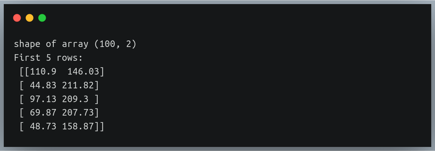
You can verify the results again by checking the shape of the data array and also printing the first few rows:

print("shape of array", data.shape)

print("First 5 rows:\n", data[:5])

Output:

Dealing with 2 delimiters

Now there may be a situation where there are more than 1 delimiters in a file.

For example, let’s imagine each of our lines contained a 3rd value representing the date of birth of the individual in dd-mm-yyyy format

110.90, 146.03, 3-7-1981
44.83, 211.82, 1-2-1986
97.13, 209.30, 14-2-1989

Now suppose we want to extract the dates, months and years as 3 different values into 3 different columns of our NumPy array. So should we pass “,” as the delimiter or should we pass “-”?

We can pass only 1 value to the delimiter parameter in the np.loadtxt method!

No need to worry, there is always a workaround. Let’s use a third file ‘./weight_height_3.txt’ for this example

We’ll use a naive approach first, which has the following steps:

  1. read the file
  2. eliminate one of the delimiters in each line and replace it with one common delimiter (here comma)
  3. append the line into a running list
  4. pass this list of strings to the np.loadtxt function instead of passing a file path.

Let’s write the code:

#reading each line from file and replacing "-" by ","
with open("./weight_height_3.txt") as f_input:

text = [l.replace("-", ",") for l in f_input]

#calling the loadtxt method with “,“ as delimiter
data = np.loadtxt(text, delimiter=",")

  • Note that we are passing a list of strings as input and not a file path.
  • When calling the function we still pass the delimiter parameter with the value “,” as we’ve replaced all instances of the second delimiter ‘-’ by a comma.
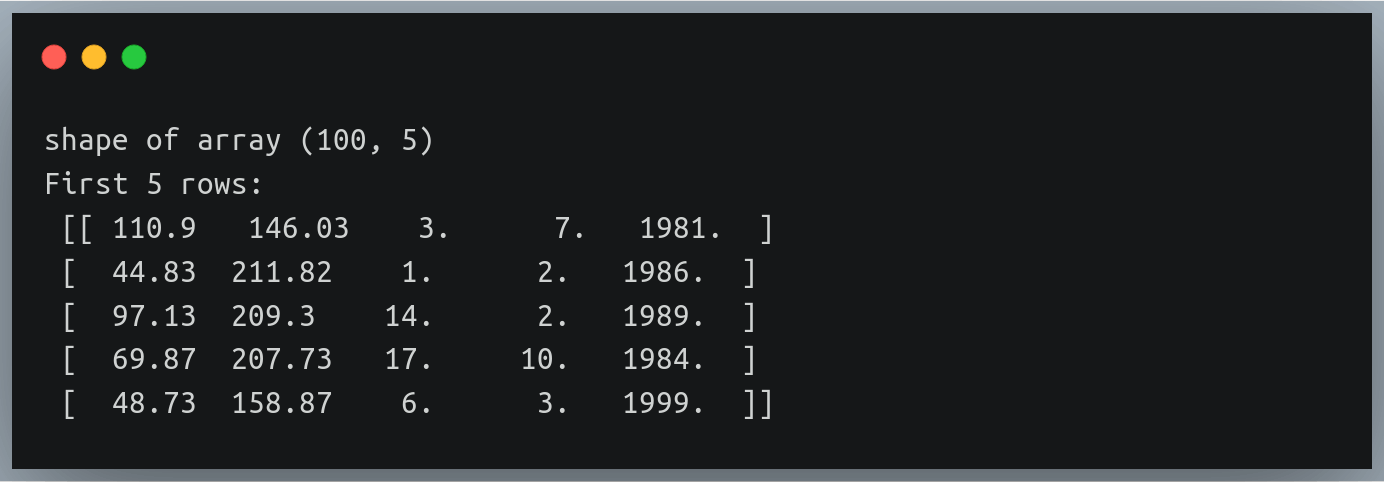
  • The returned NumPy array should now have 5 columns

You can once again validate the results by printing the shape and the first five lines:

print("Shape of data:", data.shape)

print("First five rows:\n",data[:5])

Output:

Notice how we have 3 additional columns in each row indicating the date, month and year of birth

Also notice the new values are all floating-point values; however date, month or year make more sense as integers!
We’ll look at how to handle such data type inconsistencies in the coming section.

A general approach for multiple delimiters

In this section, we will look at a general approach for working with multiple delimiters.

Also, we’ll learn how we can use generators instead of file paths – a more efficient solution for multiple delimiters, than the one we discussed in the previous section.

The problem with reading the entire file at once and storing them as a list of strings is that it doesn’t scale well. For instance, if there is a file with a million lines, storing them in a list all at once is going to consume unnecessary additional memory.

Hence we will use generators to get rid of any additional delimiter.
A generator ‘yields’ us a sequence of values on the fly i.e it will read the lines of a file as required instead of reading them all at once

So let’s first define a generator function that takes in a file path and a list of delimiters as a parameter.

def generate_lines(filePath, delimiters=[]):

with open(filePath) as f:

for line in f:

line = line.strip() #removes newline character from end

for d in delimiters:

line =line.replace(d, " ")

yield line

Here we are going through each of the delimiters one by one in each line and replacing them by a blank space ” ” which is the default delimiter in np.loadtxt function

We will now call this generator function and pass the returned generator object to the np.loadtxt method in place of the file path.

gen = generate_lines("./weight_height_3.txt", ["-",","])

data = np.loadtxt(gen)

Note that we did not need to pass any additional delimiter parameter, as our generator function replaced all instances of the delimiters in the passed list by a space, which is the default delimiter.

We can extend this idea and specify as many delimiters as needed.

Specifying the data type

Unless specified otherwise, the np.loadtxt function of the NumPy package assumes the values in the passed text file to be floating-point values by default.

So if you pass a text file that has characters other than numbers, the function will throw an error, stating it was expecting floating-point values.

We can overcome this by specifying the data type of the values in the text file using the datatypeparameter.

In the previous example, we saw the date, month and year were being interpreted as floating-point values, however, we know that these values can never exist in decimal form.

Let’s look at a new file ‘./weight_height_4.txt’ which has only 1 column for the date of birth of individuals in the dd-mm-yyyy format:

13-2-1991
17-12-1990
18-12-1986

So we’ll call the loadtxt method with “-” as the delimiter:

data = np.loadtxt("./weight_height_4.txt", delimiter="-")

print(data[:3])

print("datatype =",data.dtype)

If we look at the output of the above lines of code, we’ll see that each of the 3 values has been stored as floating-point values by default and the data type of the array is ‘float64’

We can alter this behavior by passing the value ‘int’ to the ‘dtype’ parameter. This will ask the function to store the extracted values as integers, and hence the data type of the array will also be int.

data = np.loadtxt("./weight_height_4.txt", delimiter="-", dtype="int")

print(data[:3])

print("datatype =",data.dtype)

Output:

But what if there are columns with different data types?

Let’s say we have the first two columns having float values and the last column having integer values.

In that case, we can pass a comma-separated datatype string specifying the data type of each column (in order of their existence) to the dtype parameter.

However, in such a case the function will return a NumPy array of tuples of values since a NumPy array as a whole can have only 1 data type

Let’s try this on ‘weight_height_3.txt’ file where the first two columns (weight, height) had float values and the last 3 values (date, month, year) were integers:

Output:

Ignoring headers

In some cases (especially CSV files), the first line of the text file may have ‘headers’ describing what each column in the following rows represents. While reading data from such text files, we may want to ignore the first line because we cannot (and should not) store them in our NumPy array.

In such a case, we can use the ‘skiprows’ parameter and pass the value 1, asking the function to ignore the first 1 line(s) of the text file.

Let’s try this on a CSV file – ‘weight_height.csv’:

Weight (in Kg), Height (in cm)
73.847017017515,241.893563180437
68.7819040458903,162.310472521300
74.1101053917849,212.7408555565

Now we want to ignore the header line i.e the first line of the file:

data = np.loadtxt("./weight_height.csv", delimiter=",", skiprows=1)

print(data[:3])

Output:

Likewise, we can pass any positive integer n to the skiprows parameter asking to ignore first n rows from the file.

Ignoring the first column

Sometimes, we may also want to skip the first column because we are not interested in it. For example, if our text file had the first column as “gender”, and if we don’t need to include the values of this column when extracting the data, we need a way to ask the function to do the same.

We do not have a skipcols parameter like skiprows in np.loadtxt function, using which, we could express this need. However, np.loadtxt has another parameter called ‘usecols’ where we specify the indices of the columns to be retained.

So if we want to skip the first column, we can simply supply the indices of all the columns except the first (remember indexing begins at zero)

Enough talking, let’s get to work!

Let’s look at the content of a new file ‘weight_height_5.txt’ which has an additional gender column that we want to ignore.

Male, 110.90, 146.03
Male, 44.83, 211.82


Female, 78.67, 158.74
Male, 105.64, 164.21

We’ll first determine the number of columns in the file from the first line and then pass a range of column indices excluding the first one:

with open("./weight_height_5.txt") as f:
#determining number of columns from the first line of text

n_cols = len(f.readline().split(","))

data = np.loadtxt("./weight_height_5.txt", delimiter=",",usecols=np.arange(1, n_cols))

print("First five rows:\n",data[:5])

Here we are supplying a range of values beginning from 1 (second column) and extending up to n_cols (the last column)

Output:

We can generalize the use of the usecols parameter by passing a list of indices of only those columns that we want to retain.

Load first n rows

Just as we can skip the first n rows using the skiprows parameter, we can also choose to load only the first n rows and skip the rest. This can be achieved using the max_rows parameter of the np.loadtxt method.

Let us suppose that we want to read only the first 10 rows from the text file ‘weight_height_2.txt’. We’ll call the np.loadtxt method along with the max_rows parameter and pass the value 10.

data = np.loadtxt("./weight_height_2.txt", delimiter=",",max_rows = 10)

print("Shape of data:",data.shape)

Output:

As we can see, the returned NumPy array has only 10 rows which are the first 10 rows of the text file.

If we use the max_rows parameter along with skiprowsparameter, then the specified number of rows will be skipped and next n rows will be extracted where n is the value we pass to max_rows.

Load specific rows

If we want the np.loadtxt function to load only specific rows from the text file, no parameter supports this feature.

However, we can achieve this by defining a generator that accepts row indices and returns lines at those indices. We’ll then pass this generator object to our np.loadtxt method.

Let’s first define the generator:

def generate_specific_rows(filePath, row_indices=[]):

with open(filePath) as f:

# using enumerate to track line no.
for i, line in enumerate(f):

#if line no. is in the row index list, then return that line
if i in row_indices:

yield line

Let’s now use the np.loadtxt function to read the 2nd, 4th and 100th line in the file ‘weight_height_2.txt

gen = generate_specific_rows("./weight_height_2.txt",row_indices = [1, 3, 99])

data = np.loadtxt(gen, delimiter=",")

print(data)

This should return a NumPy array having 3 rows and 2 columns:

Skip the last row

If you want to exclude the last line of the text file, you can achieve this in multiple ways. You can either define another generator that yields lines one by one and stops right before the last one, or you can use an even simpler approach – just figure out the number of lines in the file, and pass 1 less than that count to the max_rows parameter.

But how will you figure out the number of lines?
Follow along!

with open("./weight_height_2.txt") as f:

n = len(list(f))

print("n =", n)

Now n contains the number of lines present in `weight_height_2.txt` file, that value should be 100.

We will now read the text file as we used to, using the np.loadtxt method along with the max_rows parameter with value n – 1.

data = np.loadtxt("./weight_height_2.txt", delimiter=",",max_rows=n - 1)

print("data shape =",data.shape)

Output:

As we can see, the original text file had 100 rows, but when we read data from the file, it’s shape is (99, 2) since it skipped the last row from the file.

Skip specific columns

Suppose you wanted to ignore some of the columns while loading data from a text file by specifying the indices of such columns.

While the np.loadtxt method provides a parameter to specify which columns to retain (usecols), it doesn’t offer a way to do the opposite i.e specify which columns to skip. However, we can always find a workaround!

We shall first define the indices of columns to be ignored, and then using them we will derive the list of indices to be retained as the two sets would be mutually exclusive.

We will then pass this derived indices list to the usecols parameter.

Here is pseudocode for the entire process:

  1. Find the number of columns in the file n_cols (explained in an earlier section)
  2. Define the list of indices to be ignored
  3. Create a range of indices from 0 to n_cols, and eliminate the indices of step 2 from this range
  4. Pass this new list to usecols parameter in np.loadtxt method

Let’s create a wrapper function loadtext_without_columns that implements all the above steps:

def loadtext_without_columns(filePath, skipcols=[], delimiter=","):

with open(filePath) as f:

n_cols = len(f.readline().split(delimiter))

#define a range from 0 to n_cols
usecols = np.arange(0, n_cols)

#remove the indices found in skipcols
usecols = set(usecols) - set(skipcols)

#sort the new indices in ascending order
usecols = sorted(usecols)

#load the file and retain indices found in usecols
data = np.loadtxt(filePath, delimiter = delimiter, usecols = usecols)

return data

To test our code, we will work with a new file `weight_height_6.txt` which has 5 columns – the first two columns indicate width and height and the remaining 3 indicate the date, month and year of birth of the individuals.

All the values are separated by a single delimiter – comma:

110.90, 146.03, 3,7,1981
44.83, 211.82, 1,2,1986
97.13, 209.30, 14,2,1989


105.64, 164.21, 3,6,2000

Suppose we were not interested in the height and the date of birth of the individual, and so we wanted to skip the columns at positions 1 and 2.

Let’s call our wrapper function specifying our requirements:

data = loadtext_without_columns("./weight_height_6.txt",skipcols = [1, 2], delimiter = ",")

# print first 5 rows
print(data[:5])

Output:

We can see that our wrapper function only returns 3 columns – weight, month and year. It has ensured that the columns we specified have been skipped!

Load 3D arrays

So far we’ve been reading the contents of the file as a 2D NumPy array. This is the default behavior of the np.loadtxt method, and there’s no additional parameter that we can specify to interpret the read data as a 3D array.

So the simplest approach to solve this problem would be to read the data as a NumPy array and use NumPy’s reshape method to reshape the data in any shape of any dimension that we desire.

We just need to be careful that if we want to interpret it as a multidimensional array, we should make sure it is stored in the text file in an appropriate manner and that after reshaping the array, we’d get what we actually desired.

Let us take an example file – ‘weight_height_7.txt’.

This is the same file as ‘weight_height_2.txt’. The only difference is that this file has 90 rows, and each 30-row block represents a different section or class to which individuals belong.

So there are a total of 3 sections (A, B and C) – each having 30 individuals whose weights and heights are listed on a new row.

The section names are denoted with a comment just before the beginning of each section (you can check this at lines 1, 32 and 63).

The comment statements begin with ‘#’ and these lines are ignored by np.loadtxt when reading the data. We can also specify any other identifier for comment lines using the parameter ‘comments’

Now when you read this file, and print its shape, it would display (90,2) because that is how np.loadtxt reads the data – it arranges a multi-row data into 2D arrays.

But we know that there is a logical separation between each group of 30 individuals, and we would want the shape to be (3, 30, 2) – where the first dimension indicates the sections, the second one represents each of the individuals in that section and the last dimension indicates the number of values associated to each of these individuals (here 2 for weight & height).

Using NumPy reshape method

So we want our data to be represented as a 3D array.

We can achieve this by simply reshaping the returned data using NumPy’s reshape method.

data = np.loadtxt("./weight_height_7.txt",delimiter=",")

print("Current shape = ",data.shape)

Settingsdata = data.reshape(3,30,2)

print("Modified shape = ",data.shape)

print("fifth individual of section B - weight, height =",data[1,4,:])

Output:

Notice how we are printing the details of a specific individual using 3 indices

The returned result belongs to the 5th individual of section B – this can be validated from the text:

#section B
100.91, 155.55
72.93, 150.38
116.68, 137.15
86.51, 172.15
59.85, 155.53

Comparison with alternatives

While numpy.loadtxt is an extremely useful utility for reading data from text files, it is not the only one!

There are many alternatives out there that can do the same task as np.loadtxt, many of these are better than np.loadtxt in many aspects. Let’s briefly look at 3 such alternative functions.

numpy.genfromtxt

  1. This is the most discussed and the most used method alongside np.loadtxt
  2. There’s no major difference between the two, the only one that stands out is np.genfromtxt’s ability to smoothly handle missing values.
  3. In fact, NumPy’s documentation describes np.loadtxt as “an equivalent function (to np.genfromtxt) when no data is missing.
  4. So the two are almost similar methods, except that np.genfromtxt can do more sophisticated processing of the data in a text file.

numpy.fromfile

  1. np.fromfile is commonly used when working with data stored in binary files, with no delimiters.
  2. It can read plain text files but does so with a lot of issues (go ahead and try reading the files we discussed using np.fromfile)
  3. While it is faster in execution time than np.loadtxt, but it is generally not a preferred choice when working with well-structured data in a text file.
  4. Besides NumPy’s documentation mentions np.loadtxt as a ‘more flexible (than np.fromfile) way of loading data from a text file.

pandas.read_csv

  1. pandas.read_csv is the most popular choice of Data Scientists, ML Engineers, Data Analysts, etc. for reading data from text files.
  2. It offers way more flexibility than np.loadtxt or np.genfromtxt.
  3. Although you cannot pass a generator to pandas.read_csv as we did.
  4. In terms of speed of execution, however, pandas.read_csv do better than np.loadtxt

Handling Missing Values

As discussed in our section comparing np.loadtxt with other options, np.genfromtxt handles missing values by default. We do not have any direct way of handling missing values in np.loadtxt

Here we’ll look at an indirect (and a slightly sophisticated) way of handling missing values with the np.loadtxt method.

The converters parameter:

  • np.loadtxt has a converters parameter that is used to specify the preprocessing (if any) required for each of the columns in the file.
  • For example, if the text file stores the height column in centimeters and we want to store them as inches, we can define a converter for the heights column.
  • The converters parameter accepts a dictionary where the keys are column indices and the values are methods that accept the column value, ‘convert’ it and return the modified value.

How can we use converters to handle missing values?

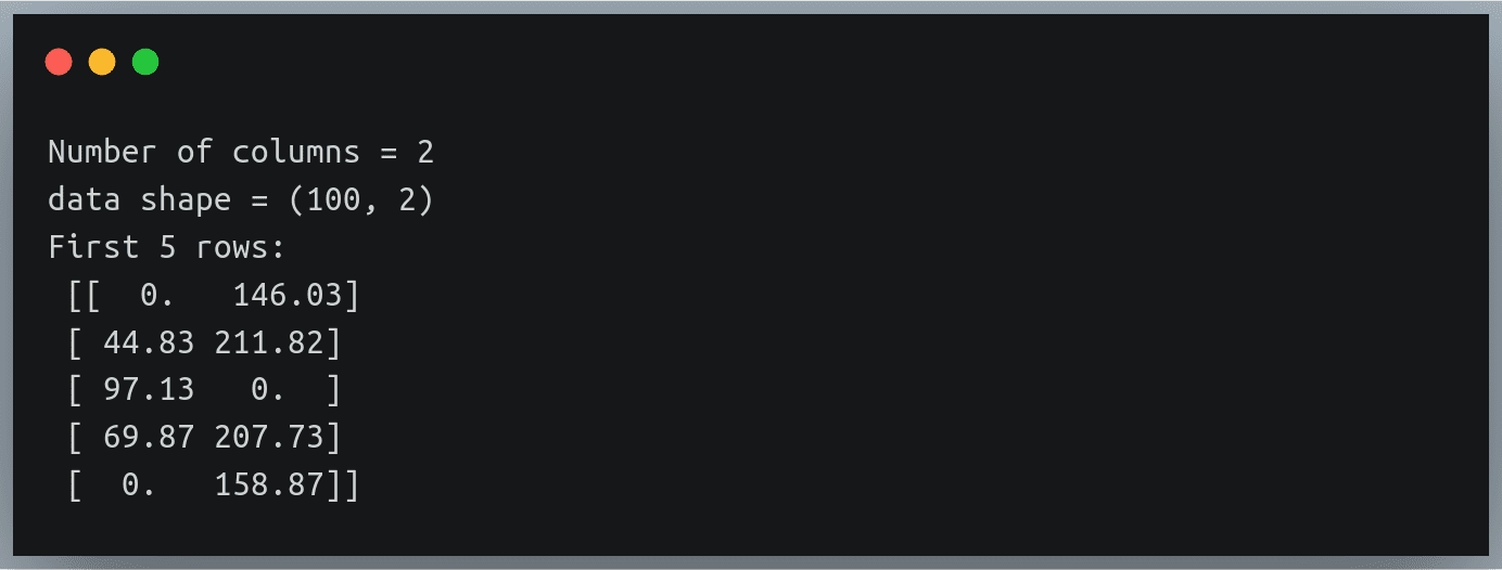
  • We need to first decide the default datatype i.e the value to be used to fill in the positions where the actual values are missing. Let’s say we want to fill in the missing height and weight values with 0, so our fill_value will be 0.
  • Next, we can define a converter for each column in the file, which checks if there is some value or an empty string in that column and if it’s an empty string, it will fill it with our fill_value.
  • To do this, we’ll have to find the number of columns in the text file, and we have already discussed how to achieve this in an earlier section.

We’ll use the file ‘weight_height_8.txt’ which is the same as ‘weight_height_2.txt’ but has several missing values.

, 146.03
44.83, 211.82
97.13,
69.87, 207.73
, 158.87
99.25, 195.41

Let’s write the code to fill in these missing values’ positions with 0.

# finding number of columns in the file
with open("./weight_height_8.txt") as f:

n_cols = len(f.readline().split(","))

print("Number of columns", n_cols)

# defining converters for each of the column (using 'dictionary
# comprehension') to fill each missing value with fill_value

fill_value = 0

converters = {i: lambda s: float(s.strip() or fill_value) for i in range(2)}

data = np.loadtxt("./weight_height_8.txt", delimiter=",",converters = converters)

print("data shape =",data.shape)

print("First 5 rows:\n",data[:5])

Output:

The missing height and weight values have been correctly replaced with a 0. No magic!

Conclusion

numpy.loadtxt is undoubtedly one of the most standard choices for reading a well-structured data stored in a text file. It offers us great flexibility in choosing various options for specifying the way we want to read the data, and wherever it doesn’t – remember there’s always a workaround!

0

10+ examples for killing a process in Linux

In this tutorial, we will talk about killing a process in Linux with multiple examples. In most cases, it’s as simple as typing “kill” command followed by the process ID (commonly abbreviated as PID).

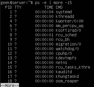
In the screenshot above, we’ve killed a process with the ID of 1813. If you are a Windows user, it may help to think of the ‘kill’ command as Linux’s equivalent of the ‘End task’ button inside of the Windows task manager. The “ps -e” command will list everything running on your system. Even with a minimal installation, the command will probably output more than 80 results, so it’s much easier to pipe the command to ‘grep’ or ‘more’.

Continue Reading →

ps -e | grep name-of-process

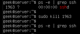
In the screenshot below, we check to see if SSH is running on the system.

Check if process is running

This also gives us the PID of the SSH daemon, which is 1963.

Pipe to ‘more’ if you want to look through your system’s running processes one-by-one.

List running processes

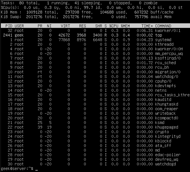
You can also make use of the ‘top’ command in order to see a list of running processes. This is useful because it will show you how many system resources that each process is using.

List processes using top command

The PID, User, and name of the resource are all identified here, which is useful if you decide to kill any of these services later.

Pay attention to the %CPU and %MEM columns, because if you notice an unimportant process chewing up valuable system resources, it’s probably beneficial to kill it!

Another very efficient away of obtaining the corresponding process ID is to use the ‘pgrep’ command. The only argument you need to supply is the name (or part of the name) of the running process.

Here’s what it looks like when we search for SSH. As you can see, it returns a process ID of 2506.

Using pgrep

Kill a process by PID

Now that we know the PID of the SSH daemon, we can kill the process with the kill command.

sudo kill 1963

Kill process by ID

You can issue a final ‘ps’ command, just to ensure that the process was indeed killed.

ps -e | grep ssh

The results come up empty, meaning that the process was shut down successfully. If you notice that the process is continuing to run – which should not normally happen – you can try sending a different kill signal to the process, as covered in the next session.

Note: It’s not always necessary to use ‘sudo’ or the root user account to end a process. In the former example, we were terminating the SSH daemon, which is run under the root user, therefore we must have the appropriate permissions to end the process.

Default signal sent by the kill command

By default, the kill command will send a SIGTERM signal to the process you specify.

This should allow the process to terminate gracefully, as SIGTERM will tell the process to perform its normal shutdown procedures – in other words, it doesn’t force the process to end abruptly.

This is a good thing because we want our processes to shut down the way they are intended.

Sometimes, though, the SIGTERM signal isn’t enough to kill a process. If you run the kill command and notice that the process is still running, the process may still be going through its shutdown process, or it may have become hung up entirely.

Force killing

To force the process to close and forego its normal shutdown, you can send a SIGKILL signal with the -9 switch, as shown here:

kill -9 processID

Force process killing

It can be tempting to always append the -9 switch on your kill commands since it always works. However, this isn’t the recommended best practice. You should only use it on processes that are hung up and refusing to shut down properly.

When possible, use the default SIGTERM signal. This will prevent errors in the long run, since it gives the process a chance to close its log files, terminate any lingering connections, etc.

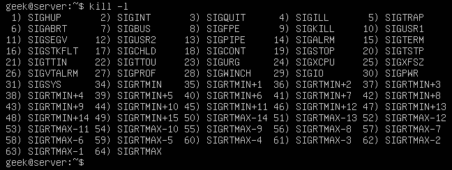
Apart from the SIGTERM and SIGKILL signals, there is a slew of other signals that kill can send to processes, all of which can be seen with the -l switch.

Kill signals

The numbers next to the names are what you would specify in your ‘kill’ command. For example, kill -9 is SIGKILL, just like you see in the screenshot above.

For everyday operations, SIGTERM and SIGKILL are probably the only signals you will never need to use. Just keep the others in mind in case you have a weird circumstance where a process recommends terminating it with a different signal.

How to kill all processes by name?

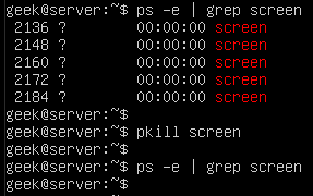
You can also use the name of a running process, rather than the PID, with the pkill command. But beware, this will terminate all the processes running the under the specified name, since kill won’t know which specific process you are trying to terminate.

pkill name-of-process

Check out the example below where we terminate five processes with a single pkill command.

Kill a process using pkill

In this example, we had wanted to only terminate one of those screen sessions, it would’ve been necessary to specify the PID and use the normal ‘kill’ command. Otherwise, there is no way to uniquely specify the process that we wish to end.

How to kill all processes by a user?

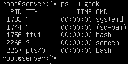
You can also use the pkill command to terminate all processes that are running by a Linux user. First, to see what processes are running under a specific user, use the ps command with a -u switch.

ps -u username

List processes running by a user

That screenshot shows us that there are currently 5 services running under the user ‘geek’. If you need to terminate all of them quickly, you can do so with pkill.

pkill -u username

pkill command

How to kill a nohup process?

The nohup process is killed in the same way as any other running process. Note that you can’t grep for “nohup” in the ps command, so you’ll need to search for the running process using the same methods as shown above.

In this example, we find a script titled ‘test.sh’ which has been executed with the nohup command. As you’ll see, finding and ending it is much the same as the examples above.

Kill nohup process

The only difference with the output is that we are notified that the process was terminated. That’s not part of kill, but rather a result from running the script in the background (the ampersand in this example) and being connected to the same tty from which the script was initiated.

nohup ./test.sh &

How to run a process in the background?

The kill command is an efficient way to terminate processes you have running in the background. You’ve already learned how to kill processes in this tutorial, but knowing how to run a process in the background is an effective combination for use with kill command.

You can append an ampersand (&) to your command in order to have it executed in the background. This is useful for commands or scripts that will take a while to execute, and you wish to do other tasks in the meantime.

Run a process in background using ampersand

Here we have put a simple ‘ls’ command into the background. Since it’s the type of command which takes very little time to execute, we’re given more output about it finishing its job directly after.

The output in our screenshot says “Done”, meaning that the job in the background has completed successfully. If you were to kill the job instead, it would show “terminated” in the output.

You can also move a job to the background by pressing Ctrl+Z on your keyboard. The ^Z in this screenshot indicates that Ctrl+Z was pressed and the test.sh script has been moved into the background.

Run a process in background using CTRL+Z

You can see test.sh continuing to run in the background by issuing a ps command.

ps -e | grep test.sh

List background processes

Using screen command

Another way to run a process in the background is to use the ‘screen’ command. This works by creating what basically amounts to a separate terminal window (or screen… hence the name).

Each screen that you create will be given its own process ID, which means that it’s an efficient way of creating background processes that can be later ended using the kill command.

Screen isn’t included on all Linux installs by default, so you may have to install it, especially if you’re not running a distribution meant specifically for servers.

On Ubuntu and Debian-based distributions, it can be installed with the following command:

sudo apt-get install screen

Once screen command is installed, you can create a new session by just typing ‘screen’.

screen

But, before you do that, it’s good to get in the habit of specifying names for your screens. That way, they are easy to look up and identify later. All you need in order to specify a name is the -S switch.

screen -S my-screen-name

Let’s make a screen called “testing” and then try to terminate it with the ‘kill’ command. We start like this:

Screen command

After typing this command and pressing enter, we’re instantly taken to our newly created screen. This is where you could start the process that you wish to have running in the background.

This is especially handy if you are SSH’d into a server and need a process to continue running even after you disconnect.

With your command/script running, you can disconnect from the screen by pressing Ctrl+A, followed by D (release the Ctrl and A key before pressing the D key).

Disconnect from screen

As you can see, screen command has listed the process ID as soon as we detached the screen. Of course, we can terminate this screen (and the command/script running inside of it), by using the kill command.

You can easily look up the process ID of your screen sessions by using this command:

screen -ls

List screen sessions

If we hadn’t named our screen session by using the -S switch, only the process ID itself would be listed. To reattach to the any of the screens listed, you can use the -r switch:

screen -r name-of-screen
or
screen -r PID

Reattach screen process

In the screenshot below, we are killing the screen session we created (along with whatever is being run inside of it), and then issuing another screen -ls command in order to verify that the process has indeed ended.

Kill screen session

How to kill a background process?

In one of our examples in the previous section, we put our tesh.sh script to run in the background. Most background processes, especially simple commands, will terminate without any hassle.

However, just like any process, one in the background may refuse to shut down easily. Our test.sh script has a PID of 2382, so we’ll issue the following command:

kill 2383

In the screenshot, though, you’ll notice that the script has ignored our kill command:

Process killing ignored

As we’ve learned already, kill -9 is the best way to kill a process that is hung up or refusing to terminate.

Force killing

How to kill stopped processes?

It can be useful to kill all your stopped background jobs at once if they have accumulated and are no longer useful to you. For the sake of example, we’re running three instances of our test.sh script in the background and they’ve been stopped:

./test.sh &

Stop a process

You can see these processes with the ps command:

ps -e | grep test.sh

List processes

Or, to just get a list of all the stopped jobs on the system, you can run the jobs command:

jobs

List stopped processes

The easiest way to kill all the stopped jobs is with the following command:

kill `jobs -ps`

Or use the -9 switch to make sure the jobs terminate immediately:

kill -9 `jobs -ps`

Kill stopped processes

The jobs -ps command will list all jobs’ PIDs running in the background, which is why we’re able to combine its output with the kill command in order to end all the stopped processes.

Kill operation not permitted

If you are getting an “operation not permitted” error when trying to kill a process, it’s because you don’t have the proper permissions. Either log in to the root account or use ‘sudo’ (on Debian distributions) before your kill command.

sudo kill PID

sudo kill permission

I hope you find the tutorial useful. Keep coming back.

0

Process Large Files Using PHP

If you want to process large files using PHP, you may use some of the ordinary PHP functions like file_get_contents() or file() which has a limitation when working with very large files. These functions rely on the memory_limit setting in php.ini file, you may increase the value but these functions still are not suitable for very large files because these functions will put the entire file content into memory at one point. Any file that has a size larger than memory_limit setting will not be loaded into memory, so what if you have 20 GB file and you want to process it using PHP? Another limitation is the speed of producing output. Let’s assume that you will accumulate the output in an array then output it at once which gives a bad user experience. For this limitation, we can use the yield keyword to generate an immediate result.

Continue Reading →

SplFileObject Class

In this post, we will use the SplFileObject class which is a part of Standard PHP Library.

For our demonstration, I will create a class to process large files using PHP.

The class will take the file name as input to the constructor:

class BigFile
{
protected $file;
public function __construct($filename, $mode = "r")
{
if (!file_exists($filename)) {
throw new Exception("File not found");
}
$this->file = new SplFileObject($filename, $mode);
}
}

Now we will define a method for iterating through the file, this method will use fgets() function to read one line at a time.

You can create another method that uses fread() function.

Read Text Files

The fgets() is suitable for parsing text files that include line feeds while fread() is suitable for parsing binary files.

protected function iterateText()
{
$count = 0;
while (!$this->file->eof()) {
yield $this->file->fgets();
$count++;
}
return $count;
}

This function will be used to iterate through lines of text files.

Read Binary Files

Another function which will be used for parsing binary files:

protected function iterateBinary($bytes)
{
$count = 0;
while (!$this->file->eof()) {
yield $this->file->fread($bytes);
$count++;
}
}

Read in One Direction

Now we will define a method that will take the iteration type and return NoRewindIterator instance.

We use the NoRewindIterator to enforce reading in one direction.

public function iterate($type = "Text", $bytes = NULL)
{
if ($type == "Text") {
return new NoRewindIterator($this->iterateText());
} else {
return new NoRewindIterator($this->iterateBinary($bytes));
}
}

Now the entire class will look like this:

class BigFile
{
protected $file;
public function __construct($filename, $mode = "r")
{
if (!file_exists($filename)) {
throw new Exception("File not found");
}
$this->file = new SplFileObject($filename, $mode);
}
protected function iterateText()
{
$count = 0;
while (!$this->file->eof()) {
yield $this->file->fgets();
$count++;
}
return $count;
}
protected function iterateBinary($bytes){
$count = 0;
while (!$this->file->eof()) {
yield $this->file->fread($bytes);
$count++;
}
}
public function iterate($type = "Text", $bytes = NULL)
{
if ($type == "Text") {
return new NoRewindIterator($this->iterateText());
} else {
return new NoRewindIterator($this->iterateBinary($bytes));
}
}
}

Parse large Files

Let’s test our class:

$largefile = new BigFile("file.csv");
$iterator = $largefile->iterate("Text"); // Text or Binary based on your file type
foreach ($iterator as $line) {
echo $line;
}

This class should read any large file without limitations Great!!

You can use this class in your Laravel projects by autoloading your class and add it to composer.json file.

Now you can parse and process large files using PHP easily.

Keep coming back.

Thank you.

0

30 Examples for Awk Command in Text Processing

In the previous post, we talked about sed command and we saw many examples of using it in text processing and we saw how it is good in this, but it has some limitations. Sometimes you need something powerful, giving you more control to process data. This is where awk command comes in. The awk command or GNU awk in specific provides a scripting language for text processing. With awk scripting language, you can make the following: a) Define variables, b) Use string and arithmetic operators, c) Use control flow and loops, d) Generate formatted reports. Actually, you can process log files that contain maybe millions of lines to output a readable report that you can benefit from.

Continue Reading →

Awk Options

The awk command is used like this:

$ awk options program file

Awk can take the following options:

-F fs     To specify a file separator.

-f file     To specify a file that contains awk script.

-v var=value     To declare a variable.

We will see how to process files and print results using awk.

Read AWK Scripts

To define an awk script, use braces surrounded by single quotation marks like this:

$ awk '{print "Welcome to awk command tutorial "}'

If you type anything, it returns the same welcome string we provide.

To terminate the program, press The Ctrl+D. Looks tricky, don’t panic, the best is yet to come.

Using Variables

With awk, you can process text files. Awk assigns some variables for each data field found:

  • $0 for the whole line.
  • $1 for the first field.
  • $2 for the second field.
  • $n for the nth field.

The whitespace character like space or tab is the default separator between fields in awk.

Check this example and see how awk processes it:

$ awk '{print $1}' myfile

The above example prints the first word of each line.

Sometimes the separator in some files is not space nor tab but something else. You can specify it using –F option:

$ awk -F: '{print $1}' /etc/passwd

This command prints the first field in the passwd file. We use the colon as a separator because the passwd file uses it.

Using Multiple Commands

To run multiple commands, separate them with a semicolon like this:

$ echo "Hello Tom" | awk '{$2="Adam"; print $0}'

The first command makes the $2 field equals Adam. The second command prints the entire line.

Reading The Script From a File

You can type your awk script in a file and specify that file using the -f option.

Our file contains this script:

{print $1 " home at " $6}

$ awk -F: -f testfile /etc/passwd

Here we print the username and his home path from /etc/passwd, and surely the separator is specified with capital -F which is the colon.

You can your awk script file like this:

{

text = " home at "

print $1 $6

}

$ awk -F: -f testfile /etc/passwd

Awk Preprocessing

If you need to create a title or a header for your result or so. You can use the BEGIN keyword to achieve this. It runs before processing the data:

$ awk 'BEGIN {print "Report Title"}'

Let’s apply it to something we can see the result:

$ awk 'BEGIN {print "The File Contents:"}

{print $0}' myfile

Awk Postprocessing

To run a script after processing the data, use the END keyword:

$ awk 'BEGIN {print "The File Contents:"}

{print $0}

END {print "File footer"}' myfile

This is useful, you can use it to add a footer for example.

Let’s combine them together in a script file:

BEGIN {

print "Users and thier corresponding home"

print " UserName \t HomePath"

print "___________ \t __________"

FS=":"

}

{

print $1 " \t " $6

}

END {

print "The end"

}

First, the top section is created using BEGIN keyword. Then we define the FS and print the footer at the end.

$ awk -f myscript /etc/passwd

Built-in Variables

We saw the data field variables $1, $2 $3, etc are used to extract data fields, we also deal with the field separator FS.

But these are not the only variables, there are more built-in variables.

The following list shows some of the built-in variables:

FIELDWIDTHS     Specifies the field width.

RS     Specifies the record separator.

FS     Specifies the field separator.

OFS  Specifies the Output separator.

ORS  Specifies the Output separator.

By default, the OFS variable is the space, you can set the OFS variable to specify the separator you need:

$ awk 'BEGIN{FS=":"; OFS="-"} {print $1,$6,$7}' /etc/passwd

Sometimes, the fields are distributed without a fixed separator. In these cases, FIELDWIDTHS variable solves the problem.

Suppose we have this content:

1235.96521

927-8.3652

36257.8157

$ awk 'BEGIN{FIELDWIDTHS="3 4 3"}{print $1,$2,$3}' testfile

Look at the output. The output fields are 3 per line and each field length is based on what we assigned by FIELDWIDTH exactly.

Suppose that your data are distributed on different lines like the following:

Person Name

123 High Street

(222) 466-1234

Another person

487 High Street

(523) 643-8754

In the above example, awk fails to process fields properly because the fields are separated by new lines and not spaces.

You need to set the FS to the newline (\n) and the RS to a blank text, so empty lines will be considered separators.

$ awk 'BEGIN{FS="\n"; RS=""} {print $1,$3}' addresses

Awesome! we can read the records and fields properly.

More Variables

There are some other variables that help you to get more information:

ARGC     Retrieves the number of passed parameters.

ARGV     Retrieves the command line parameters.

ENVIRON     Array of the shell environment variables and corresponding values.

FILENAME    The file name that is processed by awk.

NF     Fields count of the line being processed.

NR    Retrieves total count of processed records.

FNR     The record which is processed.

IGNORECASE     To ignore the character case.

You can review the previous post shell scripting to know more about these variables.

Let’s test them.

$ awk 'BEGIN{print ARGC,ARGV[1]}' myfile

The ENVIRON variable retrieves the shell environment variables like this:

$ awk '

BEGIN{

print ENVIRON["PATH"]

}'

You can use bash variables without ENVIRON variables like this:

$ echo | awk -v home=$HOME '{print "My home is " home}'

The NF variable specifies the last field in the record without knowing its position:

$ awk 'BEGIN{FS=":"; OFS=":"} {print $1,$NF}' /etc/passwd

The NF variable can be used as a data field variable if you type it like this: $NF.

Let’s take a look at these two examples to know the difference between FNR and NR variables:

$ awk 'BEGIN{FS=","}{print $1,"FNR="FNR}' myfile myfile

In this example, the awk command defines two input files. The same file, but processed twice. The output is the first field value and the FNR variable.

Now, check the NR variable and see the difference:

$ awk '

BEGIN {FS=","}

{print $1,"FNR="FNR,"NR="NR}

END{print "Total",NR,"processed lines"}' myfile myfile

The FNR variable becomes 1 when comes to the second file, but the NR variable keeps its value.

User Defined Variables

Variable names could be anything, but it can’t begin with a number.

You can assign a variable as in shell scripting like this:

$ awk '

BEGIN{

test="Welcome to LikeGeeks website"

print test

}'

Structured Commands

The awk scripting language supports if conditional statement.

The testfile contains the following:

10

15

6

33

45

$ awk '{if ($1 > 30) print $1}' testfile

Just that simple.

You should use braces if you want to run multiple statements:

$ awk '{

if ($1 > 30)

{

x = $1 * 3

print x

}

}' testfile

Or type them on the same line and separate the if statement with a semicolon like this:

While Loop

You can use the while loop to iterate over data with a condition.

cat myfile

124 127 130

112 142 135

175 158 245

118 231 147

$ awk '{

sum = 0

i = 1

while (i < 5)

{

sum += $i

i++

}

average = sum / 4

print "Average:",average

}' testfile

The while loop runs and every time it adds 1 to the sum variable until the i variables becomes 4.

You can exit the loop using break command like this:

$ awk '{

tot = 0

i = 1

while (i < 5)

{

tot += $i

if (i == 3)

break

i++

}

average = tot / 3

print "Average is:",average

}' testfile

The for Loop

The awk scripting language supports the for loops:

$ awk '{

total = 0

for (var = 1; var < 5; var++)

{

total += $var

}

avg = total / 3

print "Average:",avg

}' testfile

Formatted Printing

The printf command in awk allows you to print formatted output using format specifiers.

The format specifiers are written like this:

%[modifier]control-letter

This list shows the format specifiers you can use with printf:

c              Prints numeric output as a string.

d             Prints an integer value.

e             Prints scientific numbers.

f               Prints float values.

o             Prints an octal value.

s             Prints a text string.

Here we use printf to format our output:

$ awk 'BEGIN{

x = 100 * 100

printf "The result is: %e\n", x

}'

Here is an example of printing scientific numbers.

We are not going to try every format specifier. You know the concept.

Built-In Functions

Awk provides several built-in functions like:

Mathematical Functions

If you love math, you can use these functions in your awk scripts:

sin(x) | cos(x) | sqrt(x) | exp(x) | log(x) | rand()

And they can be used normally:

$ awk 'BEGIN{x=exp(5); print x}'

String Functions

There are many string functions, you can check the list, but we will examine one of them as an example and the rest is the same:

$ awk 'BEGIN{x = "likegeeks"; print toupper(x)}'

The function toupper converts character case to upper case for the passed string.

User Defined Functions

You can define your function and use them like this:

$ awk '

function myfunc()

{

printf "The user %s has home path at %s\n", $1,$6

}

BEGIN{FS=":"}

{

myfunc()

}' /etc/passwd

Here we define a function called myprint, then we use it in our script to print output using printf function.

I hope you like the post.

Thank you.

likegeeks.com

0